This project developed a set of high quality GIS datasets of the emergent and shallow marine features (reef boundaries, reef tops, islands, and cays) of the Coral Sea Marine Park (CSMP). The goal of this mapping was to improve the precision and spatial detail of existing reef maps. ## Features mapped: - Coral atoll platform boundary - outer visible extent (~40 - 60 m depth) - Coral reef boundary - coral substrate, plus connected sand, raised off atoll platform, mapped to 30 - 50 m depth. - Reef tops (5 m and 10 m depth) - Coral cays (above mean high water) - Coral cay vegetation - Beach rock - around coral cays and where visible on reef tops - Beach (high tide water to vegetation, excluding beach rock) - Structures (wrecks, weather stations, buildings) - incomplete coverage This project mapped reef boundaries features in a manner similar to the existing reef mapping of the Great Barrier Reef Marine Park (GBRMP) and Torres Strait (Lawrey, et al. 2016). The key characteristics of this mapping is the focus on determining the outer most boundary of coral reefs, where they rise up off the surrounding sea floor. In the Coral Sea the coral atoll platform was considered the sea floor and any solid coral structure raised up off the atoll platform was considered a coral reef. The reef boundaries also include sandy areas that connect close reef patches and surrounding sand that is highly connected to the coral substrate, as evidenced by halos (sand cleared of algae by fish around the coral patches). Patches of coral closer than 50 - 300 m were merged together to make fewer, but larger coral reef boundaries. The merge distance depended on slope, depth, structural uncertainty and visual uncertainty. The accuracy of the reef boundaries was checked by comparing digitisation of a subset of the features by independent team members. Digitised features were reviewed and refined by a second team member using additional imagery. Reef boundaries were linked with historic names based on nautical charts and historic maps, then assigned a permanent identifier that can be used instead of the reef name. Large reef features were cut into multiple segments where different sections are known by different names. In addition to reef boundary mapping the structure of the reef tops was mapped using satellite derived bathymetry to estimate a 5 and 10 metre depth boundary. The 5 m depth reef top aligns with the existing 'Dry reefs' mapping performed in the Great Barrier Reef. Shallow features were also mapped, including coral cays, surrounding beach rock and vegetation. Additionally the beach area (above high tide, but below vegetation) was mapped to provide a proxy for potential turtle nesting areas. Finally where they were visible, man made structures along with ship wrecks were mapped, however the resolution of the imagery available meant that these features were far from comprehensive. The features were digitised using a combination of satellite and drone imagery. Sentinel 2 (10 m resolution) and Landsat 8 (30 m resolution) imagery was used to map all marine features, drone imagery was used to map some of the cay areas, while the rest were mapped with publicly available ArcGIS World Imagery (~0.5 - 1m resolution). The Sentinel 2 and Landsat 8 imagery were processed into cloud free composite images using the Google Earth Engine. The imagery along with the processing scripts and mapped features are openly available.

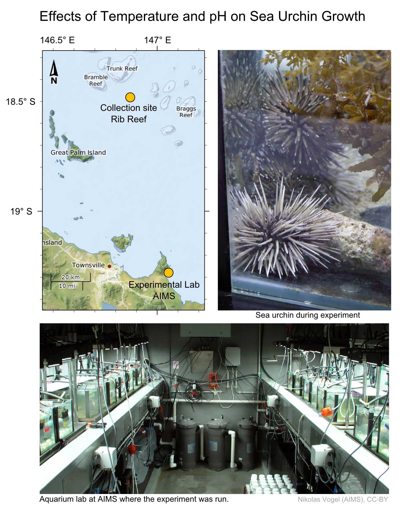
This experiment grew adult Echinometra sp. A sea urchins under four temperature and pH treatments 28 / 7.9, 28 / 8.1, 31 / 7.9, 31 / 8.1 (degrees C, pH) to investigate the interactive effects of warming and acidification on their physiology. These treatments were chosen to match those that may be experienced in the near-future (2100) due to climate change. Each treatment was replicated across 3 aquaria, each with 6 individuals for a total of 72 sea urchins. Method: The adult Echinometra sp. A used in this experiment (32–54 mm diameter, 16–68 g wet weight) were collected on the 7th of September 2011 at 2–5 m water depth at Rib Reef (146 deg 52.49’ E, 18 deg 28.86’ S), a midshelf reef in the central section of the Great Barrier Reef. They represent 'intermediate-sized' adult animals at Rib Reef, omitting the smallest and largest specimens. The experiment started three weeks after individuals were collected. The growth rate of the urchins was measured over 70 days and expressed as a percentage increase of the original weight. Sea urchins were placed into the aquaria on the 21 September 2011 (Day 0) and feed over the life of the experiment on brown macroalgae and coral rubble encrusted with crustose coralline algae was offered as an additional food source. To reduce the influence of gut contents on weight measurements were taken after a 24 hour starvation period. The six individuals in each aquarium were distinguished based on colour patterns and size, which allowed each of their individual growth rates to be measured. At the end of the experiment (Day 77) all Echinometra sp. A were dissected and the coelomic fluid carefully drained and its pH measured. The gonads were dried, weighed and sections were examined. The experiment and its results are described in more detail in: S. Uthicke, M. Liddy, H. D. Nguyen, M. Byrne (2014), Interactive effects of near-future temperature increase and ocean acidification on physiology and gonad development in adult Pacific sea urchin, Echinometra sp. A,. Coral Reefs. DOI 10.1007/s00338-014-1165-y Data Dictionary: Echinometra_Growth_righting.csv: - wt_weight_initial: Initial wet weight (grams) of the sea urchins after blotting on day 1 after 24 hour starvation. - diameter_initial: Initial diameter (mm) after blotting on day 1 after 24 hour starvation. - wt_weight_final: Final wet weight (grams) after 70 days of treatment - diameter_final: Final diameter (mm) after 70 days of treatment - righting time: Time (seconds) for the individual to right itself after being turned upside down on day 10 - weight difference: Difference between the weight before and after 70 days of treatment - growth_perc_BW: Percentage change in the weight - diameter difference: Change in the diameter of each individual after 70 days of treatment. - Aquaria: ID of the aquarium that each sea urchin was kept in. - N_pH-temp: Number of pH and temperature measurements - Temp_real: Average of measured temperatures of the aquarium over the experimental period. These were measured manually on most days (N=55) to confirm the performance of the automated temperature control. - SD_Temp_real: Standard deviation of the measured temperatures. - pH_real: Average of the measured pH of the aquarium over the experimental period. These were manually measured using a temperature-corrected pH meter (OAKTON, USA) and pH probe (EUTECH, USA). - SD_pH_real: Standard deviation of the measured pH. Echinometra_Gonad Index_noNA_actual_temps_ph.csv: - Treat: Temperature / pH treatment - Aquarium: ID of the aquarium - Urchin No: Number of the sea urchin in each tank - Sex: m - male, f - female - Temp: Temperature treatment (degrees) - pH: pH treatment - Test_diam: (cm) final diameter (mm) after blotting on day 1 after 24 hour starvation - Drained_wt with tray: Final wet weight (grams) after 70 days of treatment, including weight of tray - Gonad_wet_wt_w_tray: : Wet weight of the dry gonad plus the measuring tray. - Test_wt_weight: test-weight after subtracting tray weight. - Gonad_wt_weight: Gonad wet weight after subtracting measuring tray weight. - GI_wet: gonad index (the gonad weight as a percentage of total wet weight ) - Gonad_dry total wt: Weight of the dry gonad plus the measuring tray. - Gonad_tray_wt: Weight of the measuring tray used to weight the dry gonads - Gonad_dry_wt: Weight of the dry gonad (grams) after extraction and oven drying for 48 hours at 60 degrees C. (Gonad_dry total wt-Gonad_tray_wt) - Test_dry_weight: Weight of the urchin test in grams (Test_dry_with_tray - Tray_wt) - GI_dry: gonad index (gonad weight expressed as % of total dry weight) - Test_dry_with_tray: Weight of the urchin test + weight of the tray (grams) - Tray_wt: Weight of the tray used to take measurements of Test_dry_with_tray. - CF_pH: pH in coelomic fluid measured within 2 min of the dissection. - Gonad_dry_5 gonads: total gonad weight extrapolated to 5 gonads (only 3 were weighed for other measures because tissues were kept for other purposes) - GI_5_gonads_dry: total gonad weight extrapolated to 5 gonads (only 3 were weighed for other measures because tissues were kept for other purposes) - Temp_real: Average of measured temperatures of the aquarium over the experimental period. These were measured manually on most days (N=55) to confirm the performance of the automated temperature control. - pH_real: Average of the measured pH of the aquarium over the experimental period. These were manually measured using a temperature-corrected pH meter (OAKTON, USA) and pH probe (EUTECH, USA).

This dataset shows the concentrations of the herbicide glyphosate remaining over time in a simulation flask persistence experiment conducted in 2013. Glyphosate degradation experiments were carried out in flasks according to the OECD methods for ‘‘simulation tests’’. The tests used natural coastal seawater and were carried out in the incubator shakers under 3 conditions: (1) 25°C in the dark, (2) 31°C in the dark and (3) 25°C in the light. The light levels were ~40 µE on a 12:12 light:dark cycle and the flasks shaken at 100 rpm for up to 330 days. Water samples were taken periodically and analysed by high performance liquid chromatography-mass spectrometry (HPLC-MS/MS). Reductions in the concentration of Glyphosate were plotted to predict the persistence of this herbicide (its “half-life”). The emergence of AMPA, a breakdown product of Glyphosate, was also quantified. The experiment and its results are described in full detail in: P. Mercurio, F. Flores, J. F. Muller, S. Carter, A. P. Negri AP (2014), Glyphosate persistence in seawater. Marine Pollution Bulletin http://dx.doi.org/10.1016/j.marpolbul.2014.01.021 Data Format: The data consists of a CSV file containing the results of the 3 treatments. All concentrations in µg/L D25 = Dark 25 degrees celcius D31 = Dark 31 degrees celcius L25 = Light 25 degrees celcius Uncertainty in the analytical method for repeated inejctions into the LC-MS results in a concentration uncertainty of approximately ± 0.2 µg/L

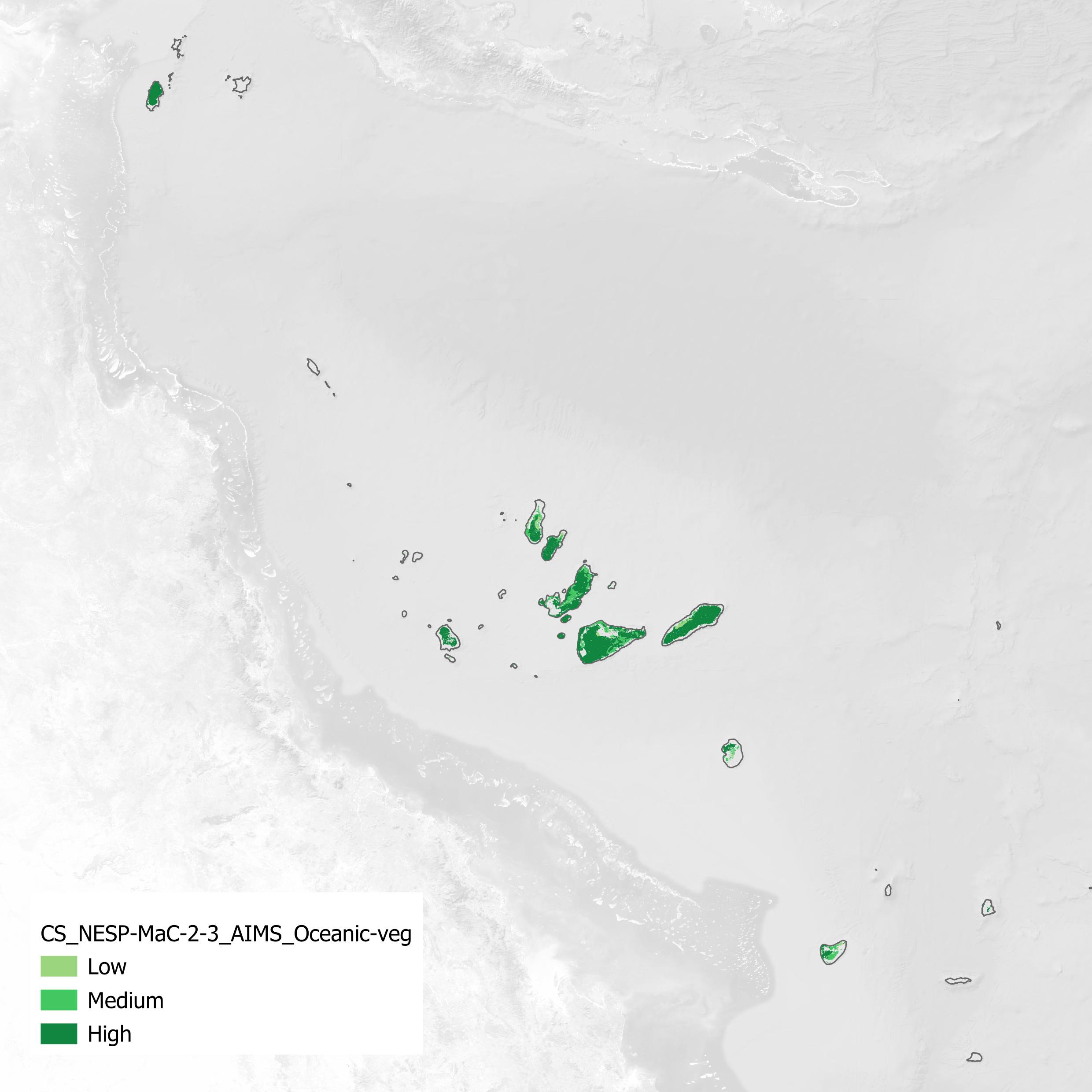
This dataset is a vector shapefile mapping the deep vegetation on the bottom of the coral atoll lagoons in the Coral Sea within the Australian EEZ. This mapped vegetation predominantly corresponds to erect macroalgae, erect calcifying algae and filamentous algae, with an average algae benthic cover of approximately 30 - 40%. Marine vegetation on shallow reef areas were excluded due to the difficulty in distinguishing algae from coral. This dataset instead focuses on the vegetation growing on the soft sediments between the reefs in the lagoons. This dataset was mapped from contrast enhanced Sentinel 2 composite imagery (Lawrey and Hammerton, 2022, https://doi.org/10.26274/NH77-ZW79). Most of the mapped atoll lagoon areas were 45 - 70 m deep. Mapping at such depths from satellite imagery is difficult and ambiguous due to there only being a single colour band (Blue B2) that provides useful information about the benthic features at this depth. Additionally satellite sensor noise, cloud artefacts, water clarity changes, uncorrected sun glint, and detector brightness shifts all make it difficult to distinguish between high and low benthic cover at depth. To compensate for some of these anomalies the benthic mapping was digitised manually using visual cues. The most important element was to identify locations where there were clear transitions between sandy areas (with a high benthic reflectance) and vegetation areas (with a low reflectance). These contrast transitions can then act as a local reference for the image contrast between light and dark substrates. These transitions were often clearest around the many patch reefs in the lagoons which have a clear grazing halo of bare sand around their perimeter. These are often then further surrounded by an intensely dark halo, presumably from a high cover of algae. These concentric rings of light and dark substrate provided local references for the image brightness of low and high benthic cover. These cues also indicated where the hard coral substrate were. These were cut out from this dataset. Validation: Since this dataset was mapped manually from noisy and ambiguous imagery it was important to establish the validity of the visual mapping approach. The manual visual mapping was based on the assumption that the higher the benthic cover of algae, the lower the benthic reflectance. The mapped vegetation therefore corresponded to locations where the benthic reflectance is low, noting that we exclude coral reef hard substrate. To verify if we could reliably map low benthic reflectance areas we first mapped North Flinders and Holmes reefs using visual techniques, then compared this with a direct estimate of benthic reflectance determined by combining the satellite imagery with high resolution bathymetry (Lawrey, 2024, https://doi.org/10.26274/s2a8-nw72). This estimate of the benthic reflectance adjusted the satellite image to the brightness and contrast levels expected for the known depths. This showed there was very strong alignment between the manual visual mapping and low benthic reflectance. The main deviations were with the fine details around reefs, and in some parts where the water clarity made it difficult to determine if the area was vegetation, deep, or water with high CDOM. Unfortunately, the high resolution bathymetry needed for the benthic reflectance estimation was not available for the rest of the Coral Sea and so it was mapped from just the manual visual mapping from the satellite imagery (Lawrey and Hammerton, 2022, https://doi.org/10.26274/NH77-ZW79) based on lessons learnt from North Flinders and Holmes reefs. The final mapped areas in Holmes, Tregrosse and Lihou Reefs were validated against a drop camera survey conducted by JCU in 2022 (yet to be published). From this 219 survey locations overlapped the atoll lagoons. Preliminary analysis indicating that areas mapped in this dataset as having high benthic vegetation typically have 15 - 70% (average 42%) algal benthic cover, typically as a mix of erect macroalgae, erect calcareous algae and filamentous algae. Lagoonal areas that were mapped as sand (i.e. areas outside the mapped vegetation, but not on a reef) typically have a much lower algal benthic cover of 0 - 22% with an average of 4%. These areas were also typically turf algae. Method: To allow the deep benthic features to be seen the blue channel of the image composites was greatly contrast enhanced to show the very faint differences in brightness due to changes in the benthos. The amount of contrast enhancement, and thus the maximum depth that could be analysed was limited by the visual anomalies in the imagery and the magnified variations in brightness across the images due to the following: - Remnant patches from masked clouds. - Remnant patches from cloud shadows that were not fully masked. - Sentinel 2 MSI detector brightness offsets. - Uncorrected tonal change across the full Sentinel swath (western side is brighter than the eastern side). - Coloured Dissolved Organic Matter in the water increases the light attenuation, making areas darker than they would appear in clear water. This tends to occur in areas with low water flushing. - Sensor noise in the imagery. - Remnant sun glint correction due to surface waves. At depth (below ~40 m), only sandy areas are visible as they reflect enough light to be visible above the surrounding visual noise. These sandy areas create a negative space around reefs and patches of dark vegetation, making their shapes visible. Most areas of the coral atoll lagoons are gently sloping meaning that sudden changes in visual brightness are likely due to changes in benthic reflectance, rather than changes in depth. We use this fact to find the visual edge of regions of low benthic reflectance (vegetation). The benthic cover (vegetation, coral or sand) was determined by manual inspection of the contrast enhanced imagery, looking for the following visual cues: - Grazing halos around patch reefs: a pale ring corresponding to bare sand surrounding a textured dark, rounded feature (patch reef). The grazing halo is typically at a similar depth to the surrounding area. This was verified by analysing bathymetry transects across patch reefs in North Flinders reef. The grazing halo therefore serves as a local brightness reference for a high benthic reflectance substrate. Often the grazing halo is surrounded by a dark halo of extra dense vegetation. This dark ring provides a brightness reference for high density vegetation. These brightness thresholds are then used to assess the density of the more distance areas around the reef. If the area is close in darkness to the dark ring around the reef then it is considered high density vegetation. If it is closer to the grazing halo bare sand then it is considered to be free of vegetation. - Reefs without grazing halos: In some cases the patch reefs do not have a pale grazing halo around them. In these cases we identify the reef by its pale circular shape, combined with evidence that it is a tall structure, by checking if it is visible in the green channel (B3), indicating that it reaches within 30 m of the surface or the available bathymetry indicates the vertical nature of the reef. These patch reefs also typically have a dark halo around them, often darker than the surrounding flat lagoonal areas. These dark rings are used as an indication of the brightness level corresponding to high density vegetation. - Low relief flat reefs: In the western side of the Tregrosse reefs platform there are quite a few dark round features that according to the bathymetry have only a limited relief of less than 8 m. These often have a small grazing halo around their border. It is unclear what the exact nature is of these reefs are, however we assume they are reefal in nature and so we exclude them from the vegetation mapping. - On the atoll plains, particularly on the western side of Tregrosse Reefs platform there are large patches of dark substrate that have clearly blank sandy patches, unrelated to the presence of reefs. In these cases the pale patches are assumed to be bare sand and serve as a high benthic reflectance guide. Limitations: This dataset was mapped at a scale of 1:400k, with our goal being to limit the maximum boundary error to 400 m. Where the imagery was clear the mapped boundary accuracy is likely to be significantly better than this threshold. The spacing of the digitised polygon vertices was adjusted to reflect the level of uncertainty in the boundary. Where visibility was good the digitisation spacing was 100 - 200 m. In high uncertainty areas the digitised distance was increased to 500 - 1000 m. The likely boundary error is approximately equal to the vertex spacing. Many of the large areas of vegetation were littered with hundreds of small patches of lower or no vegetation. These areas were cut out as holes in the digitisation where the holes were a feature larger than 200 - 300 m in size. The vegetation areas were categorised into three levels of vegetation density (Low, Medium and High) based on how dark the substrate appeared, relative to the nearby reference indicators (dark halos around reefs, and clear patches of bare sand). In practice the accuracy of this categorisation is probably quite low, as areas where only cut into these different categories at a large scale. It was very difficult to determine the extent of the vegetation in the lagoon of Ashmore Reef. The lagoon appears to have a low flushing rate and a high amount of CDOM accumulates in the lagoon, reducing the visibility to the point were most of the benthos of most of the lagoon is not visible. To help map this reef the full series of Sentinel 2 images was carefully reviewed for tonal differences that indicate the areas of sand and vegetation. Only 20% of the boundary of the vegetation could be accurately determined, the rest of the mapped boundary is speculative. Data dictionary: - Density: Estimated density of the benthic cover in three categories, Low, Medium and High. Sandy areas, or areas with very low cover were not digitised. Comparing this data to preliminary drop camera results indicates that Low and Medium correspond to an average of 30% benthic cover and High an average of 40% cover. - EdgeAcc_m: (Integer) Approximate accuracy of the feature boundary. Note that in this edition of the dataset only very few polygons were individually tagged with accuracy values. The spacing of the polygon vertices is a better local scale measure of the edge accuracy. - EdgeSrc (Edge Image Sources): (String, 255 characters) The source of the imagery used to digitise the feature or refine its boundary. - Type: Type of the feature. In this dataset all features were 'Algae'. - TypeConf: This is the confidence that the features mapped correspond to the type specified. Care was taken to exclude reefs substrate in the mapped areas, however due to the relative coarse scale of the dataset, some sandy areas and reef areas would be included in some of the polygons. - Area_km2: Area of the polygons in square kilometres. - NvclEco: Natural Values Common Language Ecosystem classification for this feature type. All features are 'Oceanic vegetated sediments'. - NvclEcoComp: Natural Values Common Language Ecosystem Complex classification. All features are 'Ocean coral reefs eAtlas Processing: No modifications were made to the data as part of publication. Location of the data: This dataset is filed in the eAtlas enduring data repository at: data\custodian\2022-2024-NESP-MaC-2\2.3_Improved-Aus-Marine-Park-knowledge\CS_NESP-MaC-2-3_AIMS_Oceanic-veg

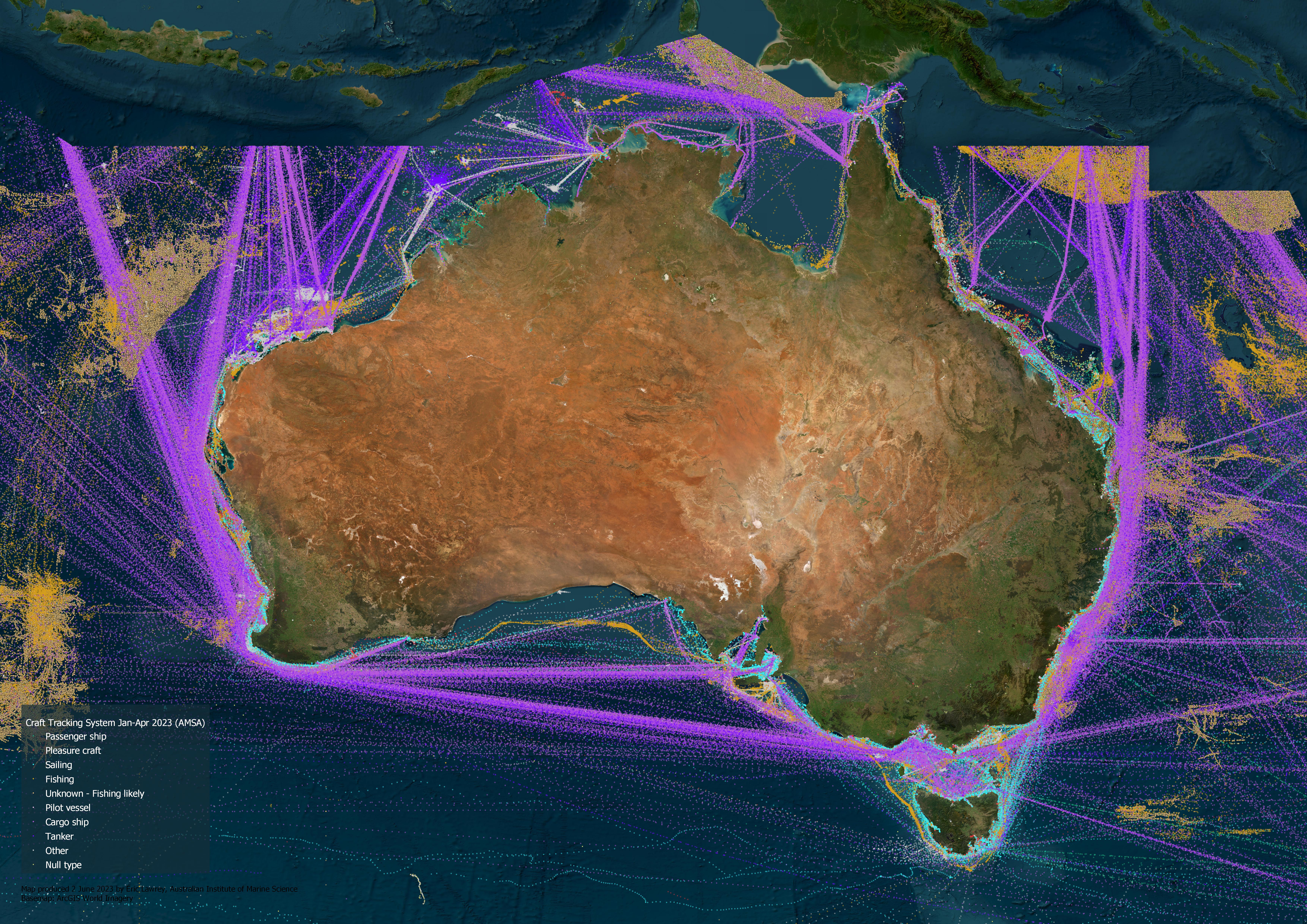
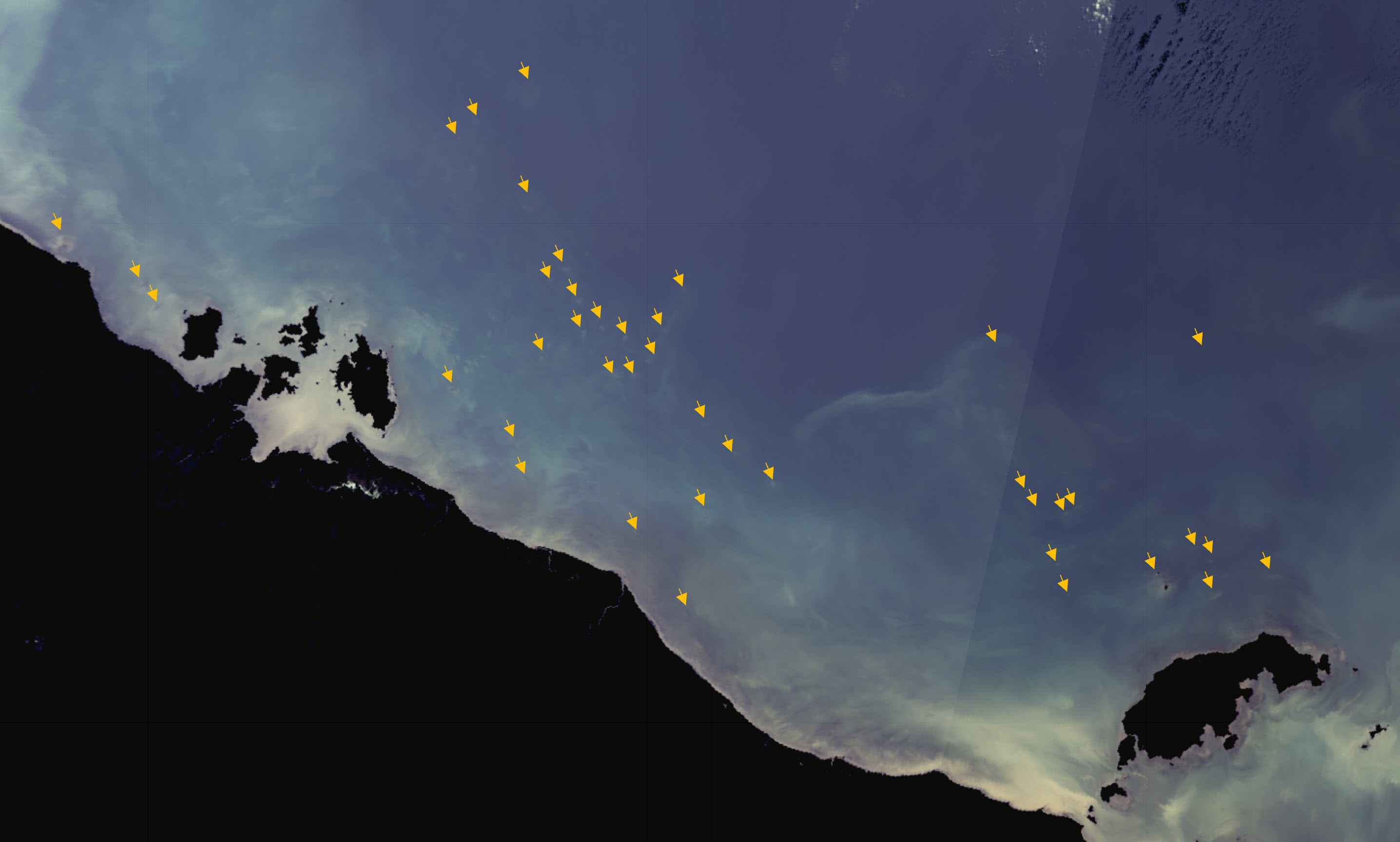
This dataset is an extract and collation of 4 months of data from the Craft Tracking System run by the Australian Maritime Safety Authority (AMSA). This dataset shows the location of cargo ships, fishing vessels, passenger ships, pilot vessels, sailing boats, tankers and other vessel types at 1 hour intervals. The Craft Tracking System (CTS) and Mariweb are AMSA’s vessel traffic databases. They collect vessel traffic data from a variety of sources, including terrestrial and satellite shipborne Automatic Identification System (AIS) data sources. This dataset has been built from AIS data extracted from CTS, and it contains vessel traffic data for January - April 2023. The dataset covers the extents of Australia’s Search and Rescue Region. Each point within the dataset represents a vessel position report and is spatially and temporally defined by geographic coordinates and a Universal Time Coordinate (UTC) timestamp respectively. This dataset is a derivative of the monthly Craft Tracking System data available from https://www.operations.amsa.gov.au/Spatial/DataServices/DigitalData. As such this record is not authoritative about the source data. If you have any queries about the Craft Tracking System data please contact AMSA. Description of the data: This data shows a high volume of cargo ships and tankers traveling between international destinations and the ports of Australia, as well as significant cargo traffic between domestic ports. These vessels tend to travel in straight lines along designated shipping lanes, or along paths that maximize their efficiency on route to their destination. Fishing activities are prominent in international waters, particularly in the Indian Ocean, Coral Sea, and Arafura Seas. The tracking of fishing vessels drops dramatically at the boundary of the Australian Exclusive Economic Zone (EEZ). Most domestic fishing activities appear to be closer to the Australian coast, often concentrating on the edge of the continental shelf. However, the data does not specifically indicate whether the vessels are domestic or international. Western Australia exhibits a great deal of vessel activity associated with the oil and gas industry. Each of these platforms is serviced by tugboats and tankers. At large ports, dozens of cargo ships wait in grid patterns to transit into the port. Shipping traffic in most of the Gulf of Carpentaria is relatively sparse, as the majority of cargo vessels travel from Torres Strait west into the Arafura Sea, bypassing the gulf. However, there is a noticeable concentration of fishing activity along the coast around Karumba and the Wellesley Islands, presumably associated with the prawning industry. Along the Queensland coastline, vessel traffic is dominated by cargo ships, which travel in designated shipping areas between the Great Barrier Reef and the mainland. There are three passages through the reef off Hay Point (Hydrographers Passage), north of Townsville (Palm Passage), and off Cairns (Grafton Passage). The Great Barrier Reef (GBR) region is frequented by pleasure crafts, sailing vessels, and passenger ships. Pleasure crafts mainly seem to visit the islands and outer reefs, while sailing vessels tend to stay within the GBR lagoon, traversing its length. Passenger ships ferry people to popular reef destinations such as reefs off the Whitsundays, Cairns, and Port Douglas, as well as Heron Island and Lady Musgrave Island. Many large passenger ships, presumably cruise vessels, travel between major ports and international destinations. These ships tend to travel 20 km further offshore than the majority of sailing boats. eAtlas Processing: The following is the processing that was applied to create this derivative dataset. This processing was functionally just a collation of 4 months of data, and a file format change (to GeoPackage) and a trimming of the length of the text attributes (which should not affect their values). Four months of data was used as this was the maximum practical limit of the rendering performance of QGIS and GeoServer. 1. The monthly CTS data was downloaded from https://www.operations.amsa.gov.au/Spatial/DataServices/DigitalData and unzipped. This data was then loaded into QGIS. 2. The `Vector / Data Management Tools / Merge Vector Layers...` tool was used to combine the 4 months of data: Input layers: cts_srr_04_2023_pt, cts_srr_03_2023_pt, cts_srr_02_2023_pt, cts_srr_01_2023_pt Save to GeoPackage: AU_AMSA_Craft-tracking-system_Jan-Apr-2023 Layername: AU_AMSA_Craft-tracking-system_Jan-Apr-2023 3. To reduce the size of the dataset the text attributes were trimmed to the length needed to store the attribute data. `Processing Toolbox > Vector table > Refactor fields` Input layer: AU_AMSA_Craft-tracking-sytem_Jan-Apr-2023 Remove attributes: layer, path (these were created by the Merge Vector Layers tool) Change: Source Expression, Original Length, New Length TYPE, 254, 80 SUBTYPE, 254, 20 TIMESTAMP, 50, 25 Refactored: AU_AMSA_Craft-tracking-system_Jan-Apr-2023_Trim.gpkg Layer name: au_amsa_craft_tracking_system_jan_apr_2023 Data dictionary: - CRAFT_ID: Double Unique identifier for each vessel - LON: Double Longitude in decimal degrees - LAT: Double Latitude in decimal degrees - COURSE: Double Course over ground in decimal degrees - SPEED: Double Speed over ground in knots - TYPE: Text Vessel type NULL 'Cargo ship - All' 'Cargo ship - Carrying DG, HS, or MP, IMO Hazard or pollutant category A' 'Cargo ship - Carrying DG, HS, or MP, IMO Hazard or pollutant category B' 'Cargo ship - Carrying DG, HS, or MP, IMO Hazard or pollutant category C' 'Cargo ship - Carrying DG, HS, or MP, IMO Hazard or pollutant category D' 'Cargo ship - No additional info' 'Cargo ship - Reserved 5' 'Cargo ship - Reserved 6' 'Cargo ship - Reserved 7' 'Cargo ship - Reserved 8' 'Engaged in diving operations' 'Engaged in dredging or underwater operations' 'Engaged in military operations' 'Fishing' 'HSC - All' 'HSC - No additional info' 'HSC - Reserved 7' 'Law enforcement' 'Local 56' 'Local 57' 'Medical transport' 'Other - All' 'Other - Carrying DG, HS, or MP, IMO Hazard or pollutant category A' 'Other - Carrying DG, HS, or MP, IMO Hazard or pollutant category B' 'Other - Carrying DG, HS, or MP, IMO Hazard or pollutant category C' 'Other - No additional info' 'Other - Reserved 5' 'Other - Reserved 6' 'Other - Reserved 7' 'Other - Reserved 8' 'Passenger ship - All' 'Passenger ship - Carrying DG, HS, or MP, IMO Hazard or pollutant category A' 'Passenger ship - Carrying DG, HS, or MP, IMO Hazard or pollutant category B' 'Passenger ship - Carrying DG, HS, or MP, IMO Hazard or pollutant category C' 'Passenger ship - Carrying DG, HS, or MP, IMO Hazard or pollutant category D' 'Passenger ship - No additional info' 'Passenger ship - Reserved 5' 'Passenger ship - Reserved 6' 'Passenger ship - Reserved 7' 'Pilot vessel' 'Pleasure craft' 'Port tender' 'Reserved' 'Reserved - All' 'Reserved - Carrying DG, HS, or MP, IMO Hazard or pollutant category B' 'Reserved - Carrying DG, HS, or MP, IMO Hazard or pollutant category C' 'Reserved - Reserved 6' 'Reserved - Reserved 7' 'Sailing' 'SAR' 'Ship according to RR Resolution No. 18 (Mob-83)' 'Tanker - All' 'Tanker - Carrying DG, HS, or MP, IMO Hazard or pollutant category A' 'Tanker - Carrying DG, HS, or MP, IMO Hazard or pollutant category B' 'Tanker - Carrying DG, HS, or MP, IMO Hazard or pollutant category C' 'Tanker - Carrying DG, HS, or MP, IMO Hazard or pollutant category D' 'Tanker - No additional info' 'Tanker - Reserved 5' 'Tanker - Reserved 6' 'Tanker - Reserved 7' 'Tanker - Reserved 8' 'Towing' 'Towing Long/Large' 'Tug' 'unknown code 0' 'unknown code 1' 'unknown code 100' 'unknown code 104' 'unknown code 106' 'unknown code 111' 'unknown code 117' 'unknown code 123' 'unknown code 125' 'unknown code 140' 'unknown code 150' 'unknown code 158' 'unknown code 2' 'unknown code 200' 'unknown code 207' 'unknown code 209' 'unknown code 223''unknown code 230' 'unknown code 253' 'unknown code 255' 'unknown code 4' 'unknown code 5' 'unknown code 6''unknown code 9' 'Vessel with anti-pollution facilities or equipment' 'WIG - All' 'WIG - Carrying DG, HS, or MP, IMO Hazard or pollutant category A' 'WIG - Carrying DG, HS, or MP, IMO Hazard or pollutant category B' 'WIG - Carrying DG, HS, or MP, IMO Hazard or pollutant category C' 'WIG - No additional info' 'WIG - Reserved 6' 'WIG - Reserved 7' - SUBTYPE: Text Vessel sub-type NULL 'Fishing Vessel' 'Powerboat' - LENGTH: Short integer Vessel length in metres - BEAM: Short integer Vessel beam in metres - DRAUGHT: Double Draught of the vessel, in metres. - TIMESTAMP: Text Vessel position report UTC timestamp in dd/mm/yyyy hh:mm:ss AM/PM format eAtlas notes: Fishing vessels are encoded as, TYPE: Fishing or TYPE: NULL, SUBTYPE: Fishing Vessel or TYPE: unknown code X. A lot of the vessels with and unknown code appeared to be predominately fishing vessels based on their behaviour. Location of the data: This dataset is filed in the eAtlas enduring data repository at: data\\non-custodian\ongoing\AU_AMSA_Craft-tracking-system

This record provides an overview of an NESP Marine and Coastal Hub research project. For specific data outputs from this project, please see child records associated with this metadata. This project will map the reefs of the northern Australian seascape, from central Western Australia, through to western Cape York in Queensland. Reefs are hotspots of conservation as they provide habitat for numerous marine species but are poorly mapped for much of northern Australia. This project will deliver datasets of reef boundaries, satellite imagery optimised for the marine environment, and geomorphic and benthic habitat maps for shallow clear reefs based on improvements to the Allen Coral Atlas. These products are targeted at assisting in the planning and evaluation of coastal development in northern Australia, helping to ensure that sensitive high value habitats are identified and considered in development proposals. This project will use satellite imaging techniques to map this region based on methods consistent with existing reef mapping of the Great Barrier Reef, Torres Strait, and the Coral Sea. Planned Outputs • Marine optimised satellite imagery for northern Australian seascape dataset (AIMS) [spatial dataset] • Reef boundary mapping for northern Australia seascape dataset (AIMS) [spatial dataset] • Improved shallow water habitat dataset (UQ) [spatial dataset] • Updated Benthic and Geomorphic Reference Data for Global Coral Reef Mapping (Western Australia, Timor Sea and Arafura Sea regions) dataset (UQ) [spatial dataset] • Technical report on Standard Operating Procedures for mapping reef boundaries (AIMS, UQ) • Final technical report with analysed data and a short summary of recommendations for policy makers of key findings [written]

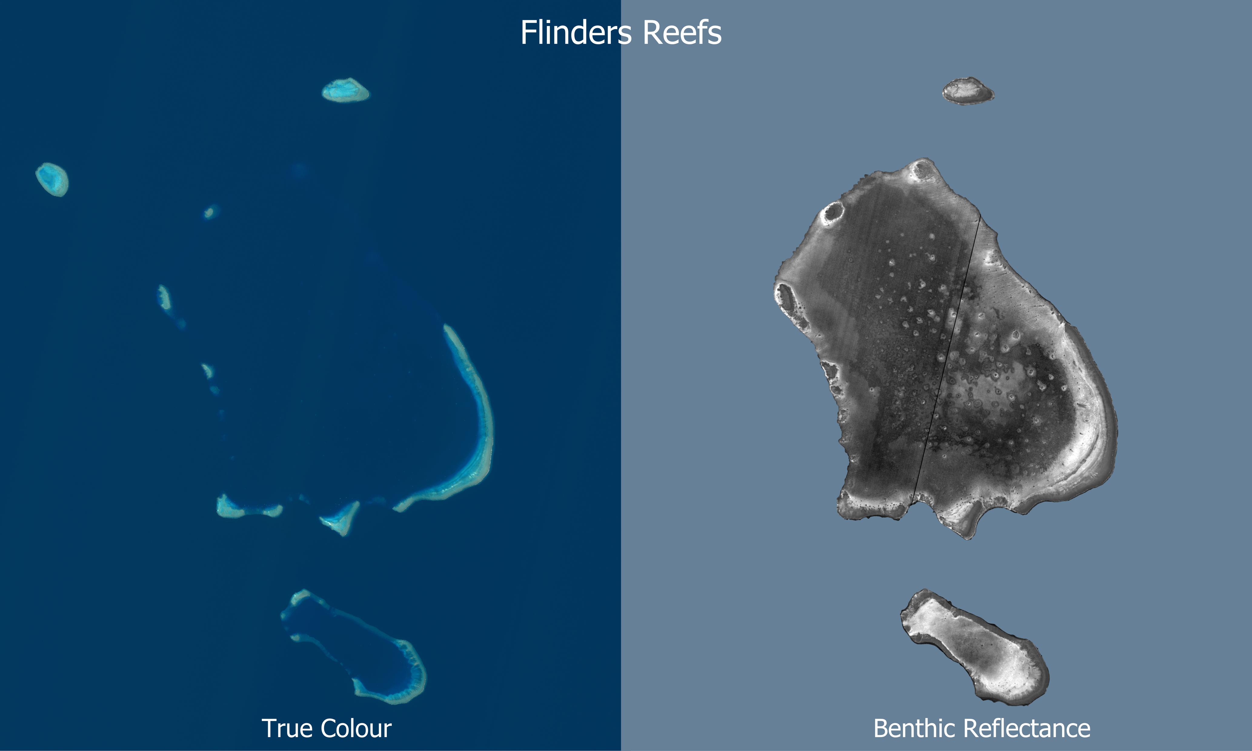
This code repository and dataset details a method for determining benthic reflectance from a combination of satellite imagery and bathymetry. Its key benefit is that it can map benthic reflectance up to 50 - 60 m in depth in clear waters, when using Sentinel 2 B2 channel combined with matching bathymetry data. Benthic reflectance is a measure of how much light the seafloor reflects and is useful for distinguishing areas that are sand (high reflectance) or vegetation such as seagrass, algae and coral (low reflectance). The proposed method allows the reflectance to be estimated much deeper than existing multi-spectral approaches that rely solely on the satellite imagery. These typically only work to depths of 10 - 20 m as they require reflected light across a wide spectral range to disentangle the depth and reflectance. In deeper areas only the blue end of the spectrum remains, making it ambiguous whether an area is dark because it is deep or dark because the substrate is dark. We resolve this ambiguity by using an independent bathymetry digital elevation model. This method only works in regions where all the following conditions are true: 1. The water is clear enough that the benthic features of interest are visible in the imagery. 2. There is a matching bathymetry dataset (with similar resolution and coverage to the satellite imagery and it is not derived from satellite imagery itself). 3. There are enough relatively flat light and dark areas that they can be used to fit the relationship between bathymetry, depth and reflectance. This dataset contains case studies for three reef complexes in the Coral Sea (Flinders Reefs, Holmes Reefs and Lihou Reefs) and a small part of the GBR north east of Townsville including Davies Reefs, Grub Reef, Chicken Reef, and Bowl Reef. It also contains additional tests to determine how sensitive the results are to degraded input data, including using a bathymetry dataset that is 1/10th the resolution (100 m) of the satellite imagery (10 m) and the effect of not performing sun glint correction prior to the benthic reflection estimation. This method was developed to assist in the mapping of oceanic vegetation on seafloor of coral atolls in the Coral Sea. For most of these atolls the available bathymetry is too low resolution and so we need to rely on manual visual mapping. This dataset serves as a visual reference where the vegetation can be mapped with greater confidence due to the estimated benthic reflectance. In this dataset we perform the same processing for each of the first four colour bands of Sentinel 2 imagery (B1 UV - 443 nm, B2 Blue - 490 nm, B3 Green - 560 nm, B4 Red - 665 nm). This is done to assess the relative effectiveness of each band and to what depth they can be used for mapping benthic reflectance. Methods: The benthic reflectance is estimated from satellite imagery and bathymetry. The satellite image brightness is scaled pixel by pixel between two thresholds corresponding to the expected brightness for low and high benthic reflectance. These thresholds are estimated from the bathymetry and a model of the depth verses brightness and benthic reflectance. This model is parameterised in each area using sampling points, chosen across the depth gradient, that have been classified as high or low benthic reflectance. The reflected light is determined by the attenuation coefficient, which is the fraction of light lost in each metre of water, the amount of scattered reflected light from deep water, and the relative brightness of the wet substrate with no water cover. This is based on the model developed by Jupp 1988. To estimate the benthic reflectance we: 1. Start with an cloud free, clear water, low noise Sentinel 2 image composite of a region and matching high resolution Digital Elevation Model (DEM) for the same region. In our case we test the approach in the Coral Sea and the GBR using Sentinel 2 image composites prepared and described in the Marine satellite image test collections (AIMS) (Lawrey and Hammerton, 2024) and the GBR 30 m and 100 m bathymetry (Beaman 2017, Beaman 2020) data sets. The GBR 30 m bathymetry covers the GBR and some of the atolls close to the GBR, including North Flinders and Holmes reefs that we use in this study. The GBR 100 m, provides coverage of the whole Coral Sea, but at a significantly lower resolution, and quality (greater levels of interpolation). 2. We manually select and record locations in the image that visually correspond to high and low benthic reflectance. In deep areas the contrast between areas that are high benthic reflectance (sand) and low benthic reflectance (vegetation or coral) is low. In these areas it is often ambiguous whether the area is dark due to depth or substrate reflectance. We therefore select sampling points where the ambiguity is low. This occurs where there is a transition between dark vegetation and sand in an area that is likely to be flat or gently sloping. 3. Each Sentinel 2 swath is imaged by 12 detectors that are staggered and overlap (MSI Overview, n.d.). In clear water areas there is a noticeable brightness difference between successive detectors in the image. Some combination of the slight differences in the sensors and parallax angle between odd and even detectors result in light and dark banding in the Sentinel 2 imagery. With the large amount of contrast stretching that is needed to estimate the benthic reflectance in deep waters, these small brightness differences can result in very large errors in the final benthic reflectance. To compensate for this we divide the Sentinel 2 imagery into sections corresponding to each of the staggered detectors in the Sentinel 2 MSI instrument, rather than whole Sentinel 2 image scenes. The depth verses image brightness modelling is performed independently on each detector. 4. We extract from the satellite imagery and the DEM triplets of bathymetry, brightness and reflectance classification. 5. We then visualise and review the depth verses brightness curves to look for outliers, then review the underlying imagery and bathymetry data for the potential reason for large deviation. To correct the outliers we would typically move the point a locations less affected the cause of the error. In most cases the errors were due to the limited resolution of the bathymetry and its errors in very shallow areas (< 1-2 m deep). We also reviewed the number of sample points in each band of depths, adding new points to improve the coverage of all depths. 6. We then fit a model for each reflectance level, and detector segment, mapping the relationship between depth and image brightness. We use a simple model, based on Jupp 1988, that assumes that the brightness of the reflected signal is the addition of scattered light plus the reflected light that exponentially decays with depth. We parameterise this model for each detector swath area based on the data established in step 4 and least squares fitting, using scipy.optimize.curve_fit. This model estimates the depth averaged attenuation coefficient for the downwelling and upwelling light for each Sentinel 2 band and the background scattered light, which largely matches the brightness of open ocean water. This model assumes that the attenuation coefficient and background scattered light is constant over the detector segment. While this model doesn't fully parameterise all the inherent optical properties of the water it does provide a very good fit under most conditions. 7. We then synthesise an estimate for the upper (corresponding to the high reflectance model) and lower (corresponding to the low reflectance model) brightness expected for each location based on the bathymetry. 8. The brightness of the original satellite imagery is then scaled between these limits, estimating the reflectance for each pixel. In deep areas the contrast is greatly enhanced scaling the high and low reflectance areas to match the contrast of shallow areas. Small errors in the model (offsets in estimates of the high and low reflectance) get magnified by the amount of contrast enhancement. To limit these errors we constrain the maximum contrast enhancement to that needed to normalise to a depth of approximately 50 m. This threshold was determined experimentally. 9. To reduce the amount of noise in the image we apply a small gaussian filter, with a filter sigma radius of 15 m (1.5 pixels in the final image). Limitations of the data: This approach only works in areas where the water is clear enough to see the benthic features and there is an independent source of high quality bathymetry. The bathymetry needs to be close in resolution to the imagery, otherwise it introduces significant errors in the conversion of satellite imagery to reflectance. In the tests performed in this study we achieve very good results using bathymetry that was three times lower resolution (30 m) than the satellite imagery (10 m). Tests using bathymetry at 1/10th the satellite imagery showed significant problems. Each area being mapped requires manually selecting points of high and low reflectance to perform the conversion. In some regions there may be insufficient high and low reflectance areas at each depth level to create the curves needed to fit the models. If the water constituents are consistent across the imagery then the scattering from suspended sediment, raising the brightness, or increases in the light absorption from coloured dissolved organic matter (CDOM), lowering the brightness, will be compensated for by the empirical sampling and modelling of the depth verses brightness for the image. If however, there is a variation in the water across the scene, such as a turbidity gradient or plumes of high CDOM coming off reefs and marine vegetation, then these brighter or darker regions will be misinterpreted by the algorithm as changes in the benthic reflectance rather than changes in water conditions. This means that any areas with a higher concentration of CDOM will be darker and falsely interpreted as having a lower benthic reflectance. Any areas that are affected by suspended sediment will be brighter and falsely interpreted by the algorithm as a higher benthic reflectance. The conversion from the satellite imagery to benthic reflectance is calibrated by manual sampling of locations across the image. These locations are classified as high or low benthic reflectance based on visual inspection of the imagery. In practice no parts of the images correspond to pure white (benthic reflectance of 1) or pure black (benthic reflectance of 0). The points labelled as high benthic reflectance typically correspond to sandy areas and low benthic reflectance areas correspond to algae or reef areas. These areas correspond to intermediate benthic reflectance values. In this study we assume that the high reflectance sampling locations correspond to a benthic reflectance of 0.8 and the low reflectance locations corresponding to a benthic reflectance of 0.4. These values are only approximate and were chosen to ensure the resulting benthic reflectance data had sufficient contrast to assist in vegetation mapping. The resulting maps are thus closer to a relative estimate of benthic reflectance than a calibrated estimate of benthic reflectance from 0 to 1. This dataset only contains a limited study area in the Coral Sea (Flinders Reefs, Holmes Reefs, Lihou Reef) and a small part of the GBR north east of Townsville including Davies Reefs, Grub Reef, Chicken Reef, and Bowl Reef. This method is appropriate for use in select locations where there is both good bathymetry and clear water. It is most useful for studying coral atolls. In this method we cut up the Sentinel 2 imagery into narrow swaths corresponding to each of the staggered detectors of the MSI instrument. We independently model the depth verses image brightness and reflectance for each of these detector swaths to compensate for the slight brightness differences in each detector swath. This however requires that there are enough useful benthic sampling sites (high and low benthic reflection) in each modelled area. Output file descriptions: This data repository contains the files used as part of the analysis including: - new-data/Depth-Reflectance-Sampling-Points.shp: This file contains 1678 manually positioned point locations across the study areas, classified as high or low reflectance. These points are used to characterize the relationship between depth, image brightness, and benthic reflectance. The points were initially placed in areas with high confidence in benthic reflectance, such as edges between sandy and vegetated areas or around grazing halos. Outliers in the brightness versus depth curves were identified and adjusted based on classification mistakes or bathymetry issues, with points moved to flatter locations when necessary. - new-data/Swath-analysis-areas-Poly.shp: This file contains areas where the brightness versus depth relationship is modeled independently. The Sentinel 2 imagery is divided into areas matching the width of each detector to account for their slightly different brightness offset characteristics, which are magnified by the benthic estimation processing. The depth versus brightness and benthic reflectance modeling is performed separately for each detector. - new-data/metadata/Benth-Reflect_dataset-bounds.shp: This contains the boundary of the dataset and is used for the creation of the dataset metadata record. It represents the extent of the study area. The following correspond to analysis results for 7 test case studies. - output/55KFA-8: North Flinders reef composite of 8 images and GBR 2020 30 m bathymetry - Reference case with clearest imagery and good bathymetry. - output/55KFA-1: North Flinders reef with single best image - To show much much difference using an image composite makes to the result. - output/55KFA-8-gbr100: North Flinders reef with lower resolution 100 m bathymetry - To show the effect of lower resolution bathymetry. - output/55KFA-8-NoSGC: North Flinders reef with an 8 image composite, but without sun glint correction - To show the benefit of sun glint correction. - output/55KEB: Holmes Reefs GBR 2020 30 m bathymetry - For comparison with JCU drop camera benthic surveys. - output/56KLF-7-gbr100: Lihou Reefs - To see the effectiveness when the bathymetry is limited. - output/55KEV: GBR north east of Townsville including Davies Reefs, Grub Reef, Chicken Reef, and Bowl Reef - To assess the performance in waters with lower water clarity and high suspended sediment than the Coral Sea. Data dictionary: The following files are available for each of the test case studies. output/*/02B-Depth_Reflect-class_S2-Bright.csv - Latitude: Location of point sample - Longitude: Location of point sample - ID: Sequential counter of point sample - Reflect: Substrate brightness, either 'High' or 'Low' - SWATH_SEG: Integer 1 or 2, corresponding to two separate areas to repeat the modelling over. - Depth_m: Bathymetry of the point sample in metres - S2_R1_B1: Sentinel 2 image brightness band 1 (UV) - S2_R1_B2: Sentinel 2 image brightness band 2 (Blue) - S2_R1_B3: Sentinel 2 image brightness band 3 (Green) - S2_R1_B4: Sentinel 2 image brightness band 4 (Red) output/03C-benthic-reflect_SEG_{swath}.tif - Estimated benthic reflectance scaled from 1 - 255. 0 is reserved for no data. References: Jupp, D. L. B., 1988. Background and extensions to Depth of Penetration (DOP) mapping in shallow coastal waters. Symposium on Remote Sensing of the Coastal Zone. Gold Coast, Queensland, Session 4, Paper 2 MultiSpectral Instrument (MSI) Overview. (n.d.). Sentinel Online. Retrieved March 8, 2024, from https://sentinels.copernicus.eu/web/sentinel/technical-guides/sentinel-2-msi/msi-instrument eAtlas Processing: No modifications were made to the data as part of publication. Location of the data: This dataset is filed in the eAtlas enduring data repository at: data\custodian\2022-2024-NESP-MaC-2\2.3_Improved-Aus-Marine-Park-knowledge\CS_NESP-MaC-2-3_AIMS_Benth-Reflect

This dataset consists of three data files (spreadsheets) from a two month aquarium experiment manipulating pCO2 and light, and measuring the physiological response (photosynthesis, growth, protein and pigment content) of the adult and juvenile stages of two species of tropical corals (Acropora tenuis and A. hyacinthus). Methods: We conducted a two-month, 24-tank experiment at AIMS’s SeaSim facility, in which recently settled juvenile- and adult-colonies of the corals Acropora tenuis and A. hyacinthus were exposed to four light treatments (high, medium, low and variable intensities), fully crossed with two levels of dissolved CO2 (400 and 900 ppm). The four light treatments used in the experiment (low, medium, high and variable) each had 12 hrs of light and a five hour ramp, but at different intensities. The high light treatment had a noon max of 500 µmol photon m-2 s-1 and a DLI of 12.6 mol photon m-2, the medium treatment had a noon max of 300 µmol photon m-2 s-1 and a DLI of 7.56 mol photon m-2, while the low light treatment had a noon max of 100 µmol photon m-2 s-1 and a DLI of 2.52 mol photon m-2. The variable treatment oscillated on a five day cycle, with four days at the low treatment intensity, a ramp day at the medium, then four days at the high treatment intensity. The mean DLI of the variable treatment was therefore the same as medium treatment. Light intensities were checked in each individual aquaria with a calibrated underwater light sensor (Licor, USA). The variable light treatment allowed us to investigate how these corals acclimate to a changing light environment, and to see if responses are due to limitation under low light, or inhibition under high light (i.e. coral responses in the variable treatment would resemble the low or high light treatments), or whether light has a cumulative effect regardless of variability (i.e. coral responses in the variable treatment would resemble the medium light treatment). Adult corals were collected from Davies Reef (18.30 S, 147.23 E) while juveniles were spawned from adults at AIMS’s SeaSim facility. After two months of experiment exposure, growth (change in corallite number) and survivorship were assessed in the juvenile corals from photographs, while growth (buoyant weight changes), and protein and pigment content were assessed in the adults after tissue stripping following standard procedures. Briefly, each adult coral nubbin was water-picked in 10 mL of ultra-filtered seawater (0.04 µm) to remove coral tissue. This tissue slurry was then homogenised and centrifuged to separate coral and symbiont components following. Total coral protein content was quantified from the coral tissue supernatant with the DC protein assay kit (Bio-Rad Laboratories, Australia), while Symbiodinium pigments in the pellet were determined spectrophotometrically (Lichtenthaler 1987, Richie 2008). Protein content was standardised to nubbin surface area, estimated with the single wax-dipping technique (Veal et al. 2010), while pigment content was standardised by nubbin surface area, as well as by protein content. A series of photophysiological measurements for the effective (PhiPSII) and maximum (Fv/Fm) quantum yield of photosystem II were made on the adults with a pulse amplitude modulated fluorometer over the final ten days of the experiment. Photosynthetic pressure (Qm: 1 - PhiPSII / Fv/Fm) and relative electron transport rate (rETR: PhiPSII * PAR) were calculated (Ralph et al. 2016) to see how they were responding to their light environment. References: Lichtenthaler HK (1987) Chlorophylls and carotenoids: Pigments of photosynthetic biomembranes. Methods in Enzymology, 148, 350–382. Ralph PJ, Hill R, Doblin MA, Davy SK (2016) Theory and application of pulse amplitude modulated chlorophyll fluorometry in coral health assessment. In: Diseases of Coral, pp. 506–523. Ritchie RJ (2008) Universal chlorophyll equations for estimating chlorophylls a, b, c, and d and total chlorophylls in natural assemblages of photosynthetic organisms using acetone, methanol, or ethanol solvents. Photosynthetica, 46, 115–126. Veal CJ, Carmi M, Fine M, Hoegh-Guldberg O (2010) Increasing the accuracy of surface area estimation using single wax dipping of coral fragments. Coral Reefs, 29, 893–897.

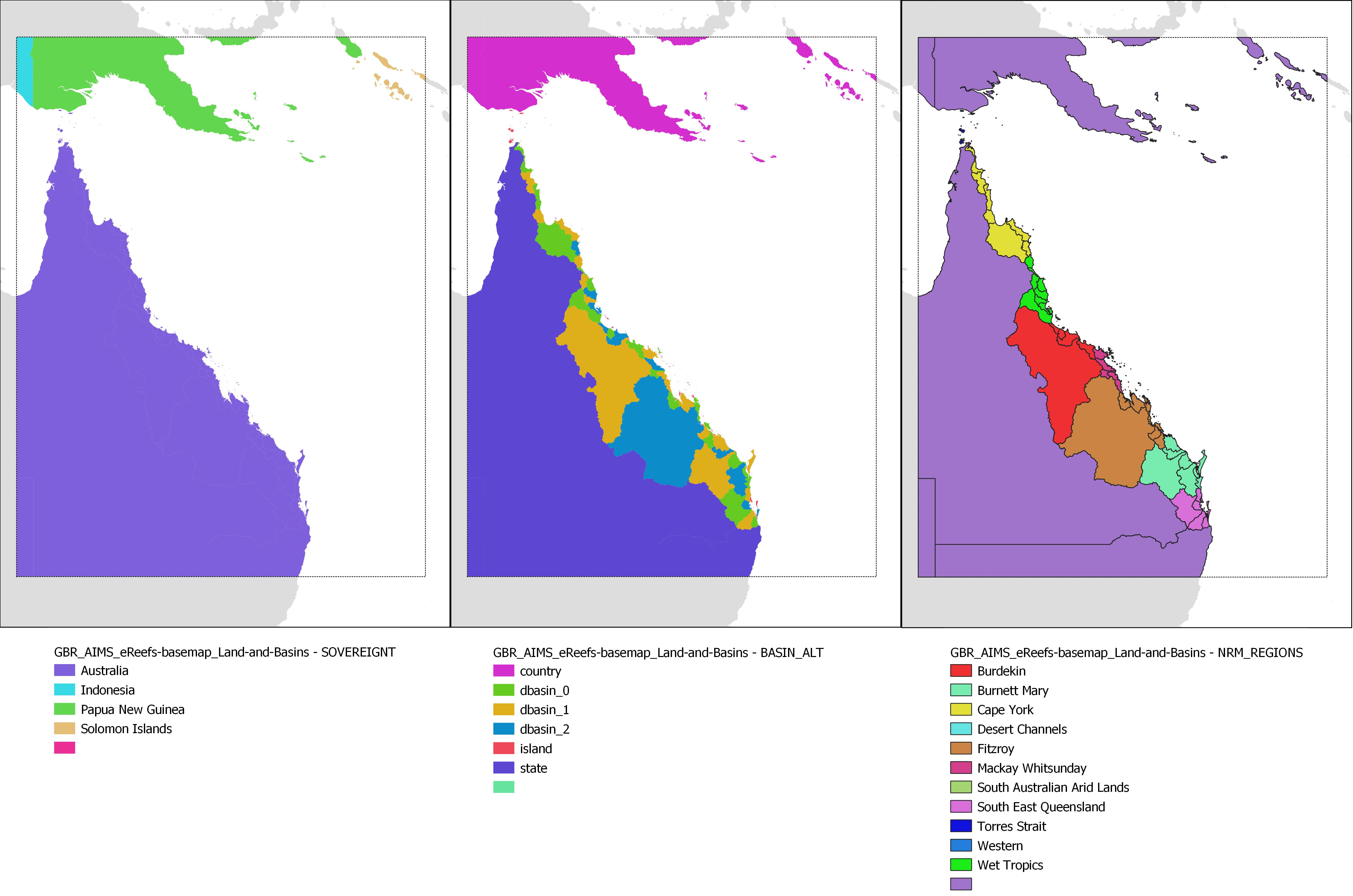
This dataset collection contains GIS layers for creating the AIMS eReefs visualisation maps (https://ereefs.aims.gov.au/). These datasets are useful for creating A4 printed maps of the Great Barrier Reef and the Coral Sea. It contains the following datasets: - Countries - Australia plus surrounding countries at 1:10M scale. Crop of Natural Earth Data 1:10 Admin 0 - Countries dataset. Allows filtering out of surrounding countries. - Cities - 21 Cities along the Queensland coastline. - Basins - Drainage basins adjacent to the Great Barrier Reef along the eastern Queensland coastline. Derived from Geoscience Australia River Basins 1997 dataset. It is a subset and reprojection. - Land and Basins - This layer contains both Queensland and PNG land areas, along with the river basins along the eastern Queensland coastline. This is an integrated layer that represents both the background land area and the river basins all in one layer. This layer saves having to map the land area, then overlay the river basins. In this way each polygon only needs to be rendered once. The goal of this layer is to optmise the rendering time of the eReefs base map. This dataset is made up from the Geoscience Australia Australia's River Basins 1997 dataset for the Queensland coastline and the eastern Queensland basins. PNG is copied from Natural Earth Data 10 m countries dataset. - Rivers - Rivers that drain along the Queensland eastern coast. This is a subset of the Geoscience Australia Geodata Topo 1:5M 2004. - Reefs - Boundaries of reefs in GBR, Torres Strait and Coral Sea. In the Coral Sea it contains the atoll platform boundaries rather than the individual reefs. This is derived from the GBRMPA GBR features dataset, AIMS Torres Strait features dataset and the AIMS Coral Sea features dataset. These were combined and simplified to a scale of 1:1M. Note that this simplification resulted in multiple neighbouring reefs being grouped together. This dataset is intended for visual rendering of maps. - Clip regions - Polygons for clipping eReefs data to the GBR. Also contains approximate polygons for Coral Sea, Torres Strait, PNG and New Caledonia. This was created principally for setting the region attribute for the Reefs dataset, but was made available as it is useful for clipping eReefs data to the GBR for plotting purposes. Methods: Most of the base map layers are derived from a variety of data sources. The full workflow used to transform these source datasets is documented on GitHub (https://github.com/eatlas/GBR_AIMS_eReefs-basemap). Limitations of the data: The datasets in this collection have been cropped and simplified for the purposes of creating low detail printed maps of the GBR. They are not intended for creating a high resolution base map. Format of the data: Shapefile and GeoJSON files. The Cities dataset is provided as a CSV file. Location of the data: This dataset is filed in the eAtlas enduring data repository at: data\custodian\2018-2024-eReefs\GBR_AIMS_eReefs-basemap

This dataset contains benthic photosynthetically active radiation (PAR; bPAR) at the Q-IMOS Myrmidon, Palm Passage and Heron Island South mooring stations from May 2016 through to November 2017. This dataset was collected to provide in situ reference data for calibration/validation of a remote sensing ocean color model to estimate bPAR (benthic photosynthetically active radiation) as part of NESP Tropical Water Quality Hub project 2.3.1. The mooring is maintained as part of the Queensland IMOS (Q-IMOS) mooring network, which collects oceanographic and water quality data at several stations. bPAR sensors were installed at four stations: Myrmidon (MYD), Palm Passage (PPS), Heron Island South (HIS) and Yongala (YGL). Methods: A WETLabs Environmental Characterization Optics (ECO) PARSB sensor was deployed and clamp-mounted to a permanent mooring wire at a fixed depth within the water column in each of three mooring sites, Myrmidon (MYD), Palm Passage (PPS), and Heron Island South (HIS). Each PAR sensor was programmed to collect 5-second blocks of data every 15 minutes. At the fourth site, Yongala (YGL), a SEABIRD SBE16PLUS V2 SEACAT profiler with PARSB auxiliary sensor “facing” upward was deployed 0.5 m above the bottom substrate. After each period of deployment, data were downloaded and the instrument’s optical component was checked, characterized and tested to ensure the quality and validity of the data between deployments. For each recovery period, the data were analysed and quality controlled such that: (i) data records in the beginning and end of each deployment were excluded to ensure that only stable PAR measurements were included in the analysis, (ii) data points when instrument failure was experienced due to instrument’s internal battery power problems were also excluded. Night-time values were forced to zero by applying an offset based on the dark count readings of the sensor for each deployment period. Summary of mooring stations and in situ data collection Mooring station: YGL Latitude: (°S) -19.302 Longitude: (°E) 147.621 Region: Shallow inshore, seasonally turbid Nominal station Depth: 30m Deployment start:19 Sep 2015 Mooring station: PPS Latitude (°S): -18.308 Longitude (°E): 147.167 Region: Deep, outer shelf, clear oceanic Nominal station Depth: 70m Deployment start: 28 May 2016 Mooring station: MYD Latitude (°S): -18.220 Longitude (°E): 147.344 Region: Deep, shelf edge, clear oceanic Nominal station Depth: 192m Deployment start: 25 May 2016 Mooring station: HIS Latitude (°S): -23.513 Longitude (°E): 151.955 Region: Shallow inshore, intermediate Nominal station Depth: 46m Deployment start: 03 Apr 2016 Data Dictionary: - bPAR: benthic photosynthetically available radiation - bPARoffset: offset (i.e., night time dark readings) corrected bPAR values Data Location: This dataset is filed in the eAtlas enduring data repository at: data\nesp2\2.3.1_Benthic-light